Lab 0 - Drama of Love
In this lab, we will use python to simulate when two people meet and fall in love. We will then use R to analyze the data and visualize the results. The goal of this lab is to get you familiar with the tools we will be using throughout the semester.
Introduction
Let’s say we have the following data
| name | gender | age | like_colors | |
|---|---|---|---|---|
| 0 | Romeo | male | 16 | red |
| 1 | Juliet | female | 14 | red |
| 2 | Hamlet | male | 30 | blue |
| 3 | Ophelia | female | 28 | pink |
we can assume that Romeo and Juliet will fall in love if their age is within 2 years of each other and they like the same color. Similarly, Hamlet and Ophelia will fall in love if their age is within 5 years of each other and they like the same color.
As this table only have 4 people, the scenario is quite simple. However, in real life, we might have hundreds or thousands of people. In this lab, we will simulate the scenario that will be more realistic.
Basic structure of a table
To producte the above table in python, we can use the following code:
import pandas as pd  # import the pandas library

names = ["Romeo", "Juliet", "Hamlet", "Ophelia"]
gender = ["male", "female", "male", "female"]
ages = [16, 14, 30, 28]
like_colors = ['red', 'red', 'blue', 'pink']

data_dict = {
    "name": names,
    "gender": gender,
    "age": ages,
    "like_colors": like_colors
}

df = pd.DataFrame(data_dict)
Here is the link from ChatGPT for explanation of the code above.
This kind of table in python and R is called a dataframe. We can think of a dataframe as a table where each row is an observation and each column is a variable. In this case, we have 4 observations and 4 variables.
Making a simulation
Now, suppose we have generate a list of 1000 people with random ages and colors they like. Names are generated randomly as well. We can write a function to match people who fall in love. The following table shows the matching results for lxlnvo.
| Name | Age | Like_Color | Gender | age_diff_with_lxlnvo | color_match_with_lxlnvo | |
|---|---|---|---|---|---|---|
| 0 | lxlnvo | 41 | yellow | Female | None | None |
| 1 | sdvkqx | 34 | orange | Male | 7 | False |
| 2 | zazcre | 20 | yellow | Male | 21 | True |
| 3 | xpksnc | 22 | indigo | Male | 19 | False |
| 4 | yiqdxn | 24 | red | Male | 17 | False |
A little bit psychology
To make our simulation more realistic, we will add five factors that could ‘define’ our personality:
- Openness: How open-minded a person is.
- Conscientiousness: How organized and responsible a person is.
- Extraversion: How outgoing and social a person is.
- Agreeableness: How kind and compassionate a person is.
- Neuroticism: How sensitive and nervous a person is.
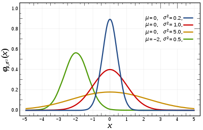
For each factor, we will assume it is a continuous variable between 0 and 100, where 0 is the lowest and 100 is the highest. We also assume that the value of each factor is normally distributed.
\[\text{Factor} \sim \mathcal{N}(\mu = 50, \sigma = 10)\]where $\mu$ is the mean and $\sigma$ is the standard deviation. We could use the following function to generate number from normal distribution:
import random

# change the value of mu and sigma to get different results
random.gauss(mu, sigma)
The following figure shows the shape of the normal distribution if you have forgotten.
Here is the result we generate:
| Name | Age | gender | openness | conscientiousness | extraversion | agreeableness | neuroticism | |
|---|---|---|---|---|---|---|---|---|
| 0 | lxlnvo | 44 | Male | 54.19 | 47.48 | 64.85 | 62.06 | 60.06 |
| 1 | sdvkqx | 58 | Female | 33.18 | 57.49 | 59.72 | 35.79 | 48.78 |
| 2 | zazcre | 42 | Female | 72.75 | 57.36 | 64.41 | 38.06 | 54.78 |
| 3 | xpksnc | 36 | Female | 48.66 | 51.99 | 60.53 | 30.53 | 52.11 |
| 4 | yiqdxn | 26 | Female | 27.98 | 49.3 | 52 | 38.64 | 49.61 |
Match people who fall in love
We will not go through the code to match people who fall in love. You will run the code in the lab session. But here are some key points:
- The simulation shows that people have higher chance to fall in love if they have more choices.
- The simulation shows that people have lower chance to fall in love if they are more picky.
- The situation becomes more complicated if we assume that people will only match with people who have higher income than them.
Do marriage make people happy?
It is tricky to answer this question. Some people say that marriage makes people happy, while others say that marriage makes people unhappy. In this lab, we will not answer this question. Instead, we will assume that happiness is a function of the following factors:
- Income: The higher the income, the happier the person is.
- Age: It follows a quadratic function, it goes down until 40 and then goes up.
- Openness: The higher the openness, the happier the person is.
- agreeableness: The higher the agreeableness, the happier the person is.
- tolerance: The higher the tolerance, the happier the person is.
Therefore the formula for happiness is:
\[\begin{aligned} \text{Happiness} & = 0.03 \times \text{Income} + 0.4 \times \text{Openness} + 0.32 \times \text{Agreeableness} \\ & \ \ \ \ \ \ \ \ \ + 0.57 \times \text{Tolerance} + 0.02 \times (\text{Age} - 40)^2 \end{aligned}\]Analyzing the data with R and data.table
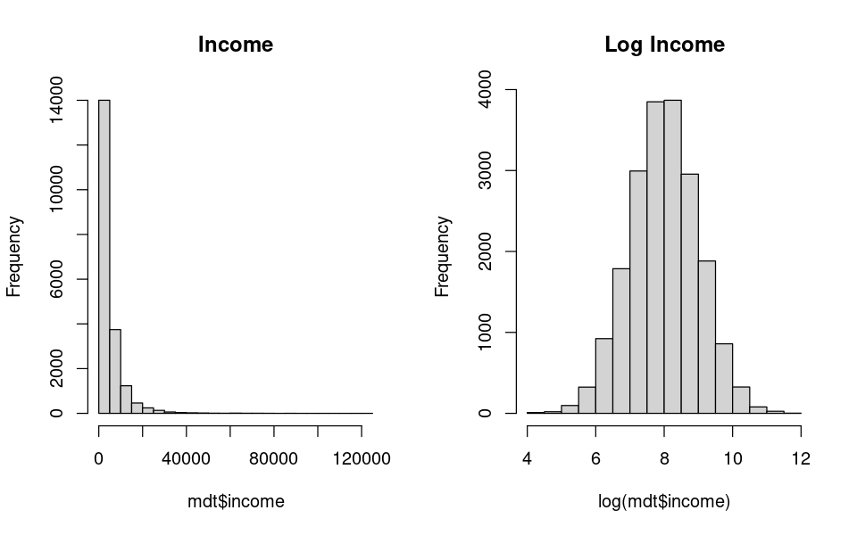
We will use R to analyze the data and visualize the results. The following code will read the data from a csv file and plot the happiness of people.
mdt <- fread("../data/marriage_data.csv")

# code to plot the distribution of income
options(repr.plot.width = 8, repr.plot.height = 5)
par(mfrow = c(1, 2))
hist(mdt$income, breaks = 20, main = "Income")
hist(log(mdt$income), breaks = 20, main = "Log Income")
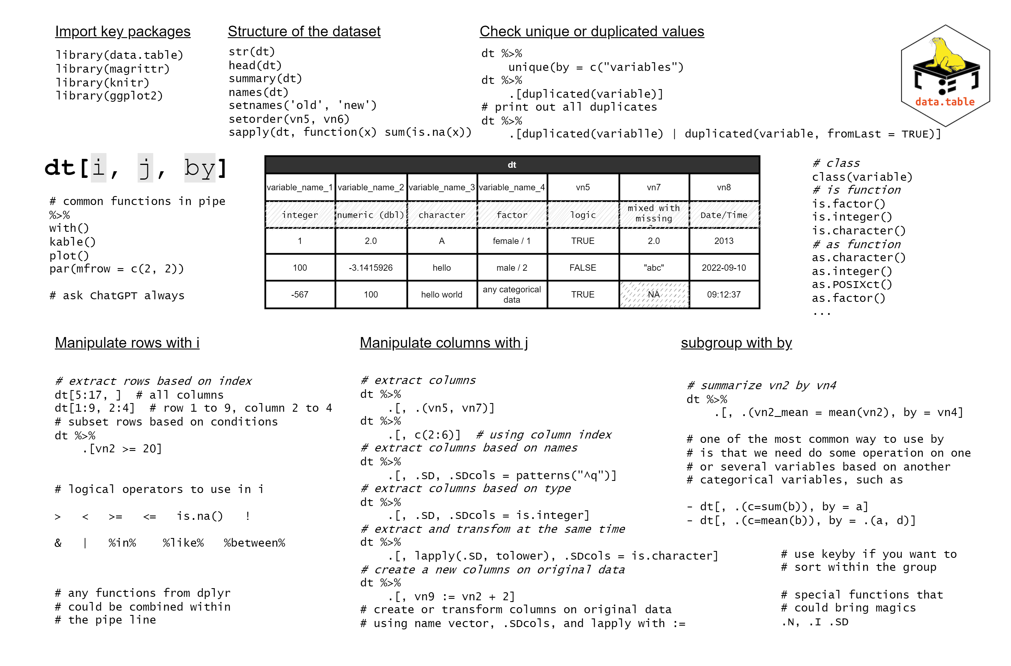
You will learn how to use R in the lab session. However it is important to know that we will use data.table package to process the data. The
data.table package is a powerful package that allows you to manipulate data in a very efficient way.
Here is the basic usage of data.table:
freadis used to read data from a csv file.dt[condition]is used to filter the data.dt[i, j, by]is used to select the data, whereiis the row condition,jis the column condition, andbyis the group by condition.
The following cheat sheet will help you to understand the basic usage of data.table. Do not worry if you do not understand it now. You will learn it in the lab session.